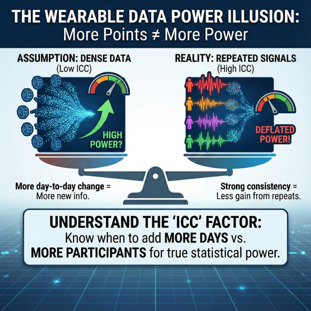
Wearable data feels inherently powerful. Continuous tracking and long follow up periods create the impression that detecting small effects should be easy.
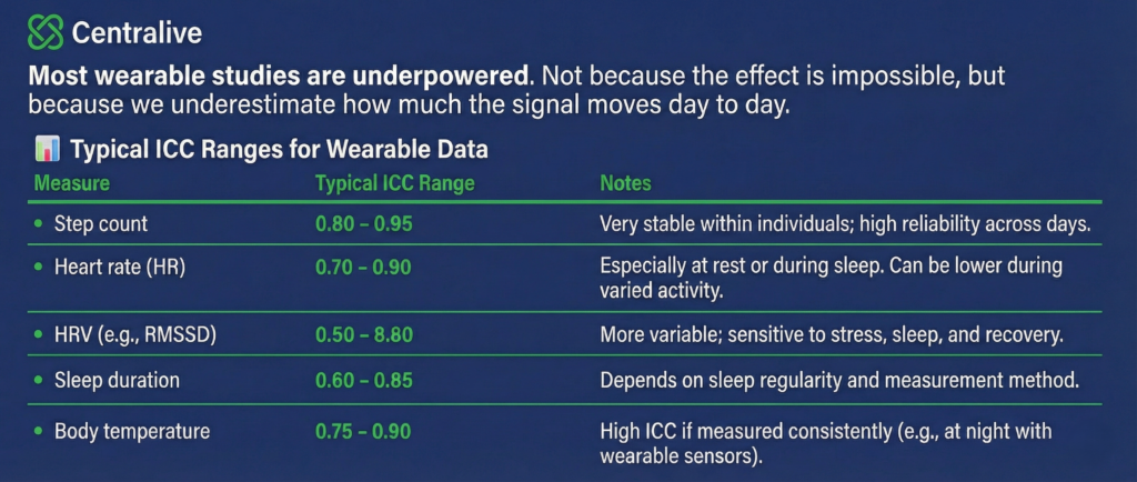
In reality, most wearable studies are underpowered. Not because the effect is impossible, but because we underestimate how much wearable signals move from day to day.
The following table shows that different wearable outcomes have very different typical ICC ranges. Step count and resting heart rate are often highly stable within individuals. HRV and sleep measures fluctuate much more. High ICC means repeated days look similar. Low ICC means each day adds genuinely new information.
This matters because statistical power depends on a simple ratio:
signal to noise = detectable change ÷ variability
For repeated measures, the variability term is dominated by within person variance, not between person differences.
The core formulas
For a simple two condition comparison with repeated measures, the standardized effect size can be written as:
d = Δ / σ
where
Δ = minimum detectable change you care about
σ = standard deviation of the outcome
With repeated measures, σ depends on ICC.
Total variance can be decomposed as:
- σ² = σ²_between + σ²_within
ICC is defined as:
ICC = σ²_between / (σ²_between + σ²_within)
Rearranging gives:
σ²_within = (1 − ICC) × σ²_total
Now consider D repeated days per participant. Averaging over days reduces within person noise:
σ²_effective = σ²_between + (σ²_within / D)
Substituting ICC:
σ²_effective = σ²_total × [ ICC + (1 − ICC) / D ]
This term directly controls power. As D increases, power improves quickly when ICC is low, and very slowly when ICC is high.
Why dense data often disappoints
The following figure illustrates the common illusion. Many wearable studies implicitly assume repeated data points are independent. In that world, power grows rapidly with more data.
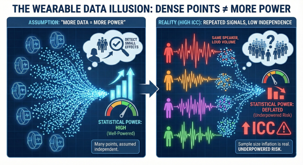
But when ICC is high, repeated points are strongly correlated. You hear the same signal again and again. Volume increases, information does not. The effective sample size grows much more slowly than expected.
That is why sample size is never just the number of participants. It is also the number of days per participant, weighted by ICC.
A concrete example
Suppose you want to detect a 5 percent increase in HRV.
Assume:
- Total standard deviation σ = 20 units
- ICC for HRV ≈ 0.5
- Target effect Δ = 5 units
Case 1: 7 days per participant
Effective variance multiplier:
ICC + (1 − ICC) / D
= 0.5 + 0.5 / 7
≈ 0.571
Effective SD:
σ_effective = 20 × √0.571 ≈ 15.1
Standardized effect size:
d = 5 / 15.1 ≈ 0.33
Case 2: 28 days per participant
ICC + (1 − ICC) / D
= 0.5 + 0.5 / 28
≈ 0.518
σ_effective = 20 × √0.518 ≈ 14.4
d = 5 / 14.4 ≈ 0.35
You gained power by adding days, but the gain was modest.
Now compare this to a high ICC outcome, say step count with ICC ≈ 0.9.
Even going from 7 to 28 days barely changes σ_effective at all. In that case, power must come from more participants, not more days.
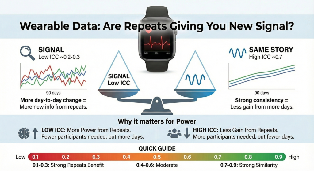
Turning theory into design choices
The following figure summarizes the tradeoff visually.
- Low ICC outcomes
Repeats are valuable. Power can come from more days per person. - High ICC outcomes
Repeats saturate quickly. Power mainly comes from more participants.
A practical workflow is:
- Pick your primary outcome
- Use prior data or literature to set a realistic ICC
- Define the smallest effect you care about
- Vary both N participants and D days in power calculations
- Choose the most feasible combination that reaches your target power
High entropy signals are often the most biologically interesting. They simply demand designs that respect their dynamics.
Centralive is built around this logic. By estimating ICC and within person variability early, teams can avoid false confidence from dense sampling and design studies that are actually powered to detect meaningful change.
Big data feels powerful. Real power comes from understanding dependency.