Suppose a participant in your study wakes up with a heart rate variability (HRV) reading 22 percent below what you recorded yesterday. Does that mean anything? Should it trigger a check-in, a survey, or a recovery prompt in your just-in-time adaptive intervention (JITAI)? Or is it simply the ordinary scatter you would expect from one night to the next?
This is one of the most common design questions we hear from researchers building HRV into remote monitoring and closed-loop interventions. The answer rarely lives in a single number. It lives in how that number compares to a person’s own recent history. This post walks through why rolling-window methods have become the standard approach for interpreting HRV, what the evidence says about choosing a window length, and how to define a deviation worth acting on.
Why a single HRV reading tells you very little
Most wearables report HRV as RMSSD (the root mean square of successive differences between heartbeats) or its natural log, lnRMSSD. Three properties of this signal make any single measurement hard to interpret on its own.
First, HRV is intensely individual. Between-person differences are dominated by age, genetics, and fitness, so a value that is perfectly healthy for one person would be alarming for another. Population reference ranges cannot tell you whether today’s reading is unusual for a given individual. The only meaningful comparison is against that person’s own baseline.
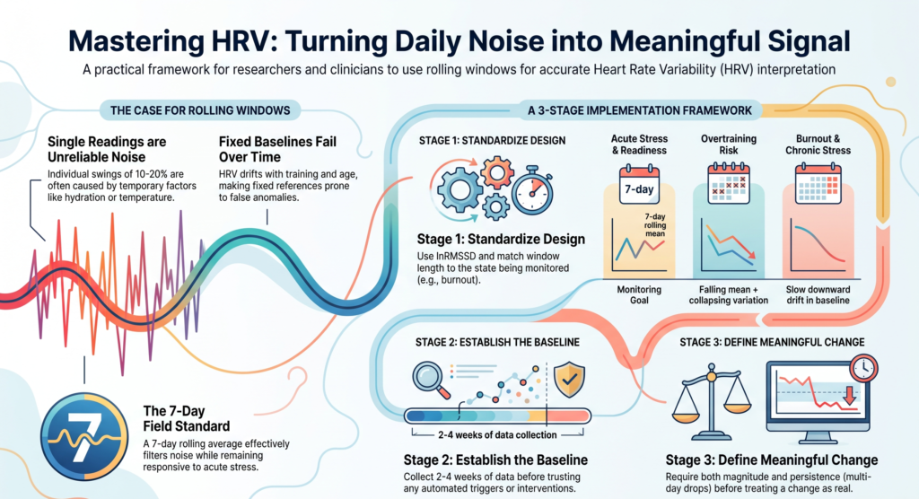
Second, day-to-day variability within the same person is large even under well-controlled conditions. Reported within-person coefficients of variation for lnRMSSD run from roughly 3 to 13 percent depending on the protocol. A 16-week validation study in Olympic water polo athletes found a mean weekly lnRMSSD coefficient of variation of 5.4 percent, sitting comfortably inside that range.1 Sleep, alcohol, hydration, room temperature, breathing pattern, measurement timing, and posture all move a single reading. A swing of 10 to 20 percent from one day to the next is frequently just noise.
Third, raw RMSSD is right-skewed. Taking the natural log pulls the distribution toward normal in most populations, which is what makes standardized comparisons such as z-scores and symmetric threshold bands interpretable. This is why the literature so consistently works with lnRMSSD rather than raw RMSSD for longitudinal monitoring.2
Put together, these three properties mean a lone measurement carries a low signal-to-noise ratio. A rolling window addresses all three at once: the rolling mean gives each person an adaptive personal baseline, and the rolling standard deviation quantifies how much scatter is normal for that person, which is exactly the information you need to judge whether a new reading is surprising.
Why a rolling baseline beats a fixed one
A tempting shortcut is to average the first two weeks of data and treat that as a fixed reference for the rest of the study. This fails because HRV drifts. A positive training adaptation, a seasonal change, a new medication, or a gradual shift in life circumstances will move the true baseline over weeks. A fixed reference would eventually flag a healthy new normal as an anomaly, or miss a genuine decline because the goalposts never moved.
A rolling baseline adapts. The common approach is to establish an initial reference period, then maintain a moving average (most often over 7 days) that updates each day. The reading you care about is always compared against the person’s recent self, not against who they were a month or a season ago.
Choosing a window length: responsiveness versus stability
Window length is a bias-variance tradeoff. A shorter window (or a single day) responds quickly to genuine change but carries more noise. A longer window is more stable but lags, and it can smooth over an acute event you would have wanted to catch. There is no universally correct length, only a length matched to the timescale of the state you are trying to detect.
The 7-day rolling average of lnRMSSD has become the field standard, largely through athlete-monitoring research. Plews and colleagues established that weekly averages track training adaptation more closely than single measures, and later showed that a minimum of about three validly timed readings per week is enough to approximate a full-week average.3 That last point is practically important for remote studies, where perfect daily adherence is rare. You do not need seven readings to compute a usable 7-day window; three well-spaced readings will often do.
The rough mapping from state to window length looks like this:
- Acute stress, daily recovery, and readiness: a 7-day rolling window is the default. It is responsive enough to register a hard week, a bout of illness, travel, or a stressful event within a day or two, while filtering out single-night noise.
- Overtraining and non-functional overreaching: track both the 7-day rolling mean and its coefficient of variation across several weeks. A jointly falling mean and collapsing variation is a recognized early-warning pattern.4
- Burnout and chronic stress: extend the observation to weeks or months. The signal here is a slow downward drift in the baseline rather than an acute dip, and as we discuss below, it is weaker and should never stand alone.
- Sleep and recovery: a 7-night rolling window of nocturnal HRV tends to be more stable than waking readings because sleep removes much of the behavioral noise, though individual nights can still swing 15 to 25 percent.
When you are unsure, a practical tactic is to run two candidate windows (say 7-day and 14-day) in parallel during piloting and compare how each trades true detections against false alarms in your specific cohort before committing to one.
Defining a deviation worth acting on
Once you have a rolling baseline and a measure of normal scatter, you can define what counts as a meaningful change. Three interoperable methods appear in the literature.
The smallest worthwhile change approach, drawn from sports science, sets a band at roughly plus or minus 0.5 times the individual’s between-day standard deviation of lnRMSSD. A rolling mean that drops below the lower edge of that band counts as a meaningful suppression. In HRV-guided training trials, this is the logic used to decide whether to prescribe a hard session or a rest day.5
The z-score or normal-range approach flags a reading when it falls outside the personal band, for example beyond one standard deviation from the rolling mean. Because lnRMSSD is approximately normal, this is straightforward to compute and to explain.
Finally, persistence and corroboration heuristics guard against acting on noise. Many consumer platforms treat a 10 to 20 percent deviation as ordinary, and reserve concern for a sustained 20 to 30 percent drop, or three or more consecutive days below baseline, ideally alongside a second signal such as elevated resting heart rate. These particular cutoffs are pragmatic rather than clinically validated, so treat them as starting points to tune in your own data, not as settled thresholds.
The unifying principle across all three: require either magnitude (clearly beyond the noise band) or persistence (sustained across days), and where possible corroborate with an independent signal, before you treat a change as real.
What the evidence actually supports
The strongest and most mature evidence for rolling-window HRV comes from endurance-athlete monitoring. A randomized trial in recreational runners scheduled harder sessions only when morning HRV sat within each runner’s individually determined worthwhile-change band. The HRV-guided group completed significantly fewer moderate and high-intensity sessions (13.2 versus 17.7, p = 0.021) yet improved 3,000 meter running performance more than a group following a fixed plan.5 A meta-analysis of HRV-guided training found a small but positive and statistically significant advantage over conventional programming.6
For burnout and chronic occupational stress, the picture is real but more modest. In the prospective Dresden Burnout Study, baseline vagally-mediated HRV inversely predicted burnout symptoms roughly a year later, and high emotional exhaustion predicted a later decline in HRV, pointing to a bidirectional relationship.7 Clinical burnout patients show lower HRV than healthy controls across most measures.8 But two major systematic reviews concluded that while the association between reduced vagal HRV and job stress is consistent, the burnout-specific association is weaker, and neither review could compute a pooled effect size because the primary studies did not report harmonized statistics.910 The practical implication is direct: for burnout, use longer observation windows and treat HRV as a complement to validated questionnaires, never as a standalone marker.
Fitting rolling-window HRV into a JITAI
In the JITAI framework, a rolling HRV deviation is a natural candidate for a passive tailoring variable that indexes a state of vulnerability, feeding a decision rule at a defined decision point such as each morning after the overnight reading. A rule might read: if the 7-day rolling lnRMSSD stays below the lower worthwhile-change bound for two or more consecutive days and resting heart rate is elevated, offer a recovery or stress-management option.
Two cautions are worth building in from the start. First, HRV speaks to vulnerability (is an adverse state present?) but not to receptivity (can the person actually engage right now?). Detecting a suppressed HRV does not tell you whether the moment is right to intervene, so contextual signals such as time, location, and activity still matter. Second, passive-sensing JITAIs in mental health remain largely at the pilot stage, and the field’s overall effect sizes are small so far. Decision rules built on rolling HRV are best treated as hypotheses to be optimized, for example through a microrandomized trial, rather than as validated triggers.
Measurement quality decides everything upstream
None of the above works if the underlying measurements are inconsistent. Standardize the device, the posture, the time of day, and the metric across the whole study. Morning supine RMSSD and nocturnal RMSSD both show good reliability; readings taken standing, during daytime activity, or in the frequency domain are far more sensitive to conditions. Nocturnal measurement has become popular precisely because sleep removes much of the behavioral confounding.
Two hard rules: never compare across devices, and never compare RMSSD-based values against SDNN-based ones. Different platforms report different underlying metrics, and mixing them invalidates the comparison. It is also worth remembering that consumer wearables produce photoplethysmography-based estimates rather than ECG, so the quality of the beat-to-beat interval series feeding your rolling window depends heavily on how cleanly those intervals are derived. Aggregating nocturnal readings over longer windows with a strict artifact threshold improves agreement with ECG considerably.11
A staged decision framework
Stage 1, study design. Decide the state you are detecting and match the window to its timescale (7 days for acute stress and recovery, weeks to months for burnout). Fix the measurement conditions and the reported metric. Plan for at least three to five readings per week rather than assuming perfect daily adherence.
Stage 2, data collection and baselining. Collect two to four weeks of standardized lnRMSSD before trusting any trigger, extending toward two months for a robust normal range. Compute the rolling mean, rolling standard deviation, worthwhile-change band, and coefficient of variation per participant. If a participant’s coefficient of variation is high (above roughly 10 to 13 percent) or their data are sparse, lengthen the window or increase reading frequency before relying on it.
Stage 3, analysis and triggering. Define the deviation with a primary rule (worthwhile-change band or z-score) and add persistence and corroboration to control false positives. Log context such as alcohol, travel, illness, and menstrual phase so a known stressor is not misread as a clinical signal. If false alarms run high during piloting, widen the band, require more consecutive days, or add a second signal, and for burnout confirm that HRV drift actually tracks your validated burnout scales in this cohort before deploying it.
The short version
Interpret HRV against a person’s own rolling baseline, not a single reading and not a fixed cutoff. Use a 7-day window as the default for acute states and longer windows for slow-moving ones like burnout. Define a meaningful deviation statistically, using a worthwhile-change band or z-score, and demand either magnitude or persistence, ideally with a corroborating signal, before you act. Above all, keep measurement conditions consistent and remember that the quality of your rolling window is only ever as good as the beat-to-beat data underneath it.
References
- Bellenger CR, et al. Common Methods and Considerations for the Analysis of Heart Rate Variability in Sleep. Sensors. 2022;22(18):6723. https://doi.org/10.3390/s22186723
- Plews DJ, Laursen PB, Stanley J, Kilding AE, Buchheit M. Training adaptation and heart rate variability in elite endurance athletes: opening the door to effective monitoring. Sports Medicine. 2013;43(9):773-781. https://doi.org/10.1007/s40279-013-0071-8
- Plews DJ, Laursen PB, Kilding AE, Buchheit M. Heart rate variability in elite triathletes, is variation in variability the key to effective training? A case comparison. European Journal of Applied Physiology. 2012;112(11):3729-3741. https://doi.org/10.1007/s00421-012-2354-4
- Plews DJ, Laursen PB, Le Meur Y, Hausswirth C, Kilding AE, Buchheit M. Monitoring training with heart rate variability: how much compliance is needed for valid assessment? International Journal of Sports Physiology and Performance. 2014;9(5):783-790. https://doi.org/10.1123/ijspp.2013-0455
- Vesterinen V, Nummela A, Heikura I, et al. Individual endurance training prescription with heart rate variability. Medicine and Science in Sports and Exercise. 2016;48(7):1347-1354. https://doi.org/10.1249/MSS.0000000000000910
- Granero-Gallegos A, Gonzalez-Quilez A, Plews D, Carrasco-Poyatos M. HRV-based training for improving VO2max in endurance athletes: a systematic review with meta-analysis. International Journal of Environmental Research and Public Health. 2020;17(21):7999. https://doi.org/10.3390/ijerph17217999
- Wekenborg MK, Hill LK, Thayer JF, et al. The longitudinal association of reduced vagal tone with burnout. Psychosomatic Medicine. 2019;81(9):791-798. https://doi.org/10.1097/PSY.0000000000000750
- Lennartsson AK, Jonsdottir I, Sjors A. Low heart rate variability in patients with clinical burnout. International Journal of Psychophysiology. 2016;110:171-178. https://doi.org/10.1016/j.ijpsycho.2016.08.005
- Jarczok MN, Jarczok M, Mauss D, et al. Autonomic nervous system activity and workplace stressors: a systematic review. Neuroscience and Biobehavioral Reviews. 2013;37(8):1810-1823. https://doi.org/10.1016/j.neubiorev.2013.07.004
- de Looff PC, Cornet LJM, Embregts PJCM, Nijman HLI, Didden HCM. Associations of sympathetic and parasympathetic activity in job stress and burnout: a systematic review. PLOS ONE. 2018;13(10):e0205741. https://doi.org/10.1371/journal.pone.0205741
- Cao R, Azimi I, Sarhaddi F, et al. Accuracy assessment of Oura ring nocturnal heart rate and heart rate variability. Sensors. 2024;24(23):7475. https://doi.org/10.3390/s24237475
Sign up for the Centralive Newsletter: https://newsletter.centralive.health/signup